Time for more height (2): but what if there is a constraint?

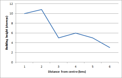
In my blog of  21 October 2018  I developed a thought experiment of how the city redeveloped in a series of steps as buildings aged and land values rose. The result is a ‘southern alps’ type  profile of building density / height (as they respond to increased land value). The tallest buildings are not necessarily in the middle of the city, and the profile of height (or density) is not a smooth curve from the centre to the fringe.

In short, while land values may present a smooth curve from centre to edge, with some ups and downs around sub regional hubs, the city skyline is jagged.

A question prompted by the exercise was what if one area of the imaginary city had a constraint placed on it? What if a height limit, density control or similar meant that buildings could not be built to a height that is reflective of the land values present? The height profile will be different in the area affected by the constraint.

Often when considering a planning constraint  we get presented with a figure similar to the one below. Rather than a smooth curve of reducing land value as distance increases, there is a disruption created by a planning constraint. In this case the constraint is represented by the grey bar. The constraint creates a ‘cliff’ along the curve.

An urban boundary control may be one example of a constraint: land on the inside of the urban fence is worth much more than land on the outside. A similar difference might come about by the constraint being a viewshaft that limits height or perhaps a special character area that limits new buildings.

The difference in land values at the constraint boundary is often taken to be the ‘cost’ of the constraint. In my made up example, on one side of the constraint, land is worth 200 units per square metre, while on the other side, land is 450 units, more than a halfing of ‘value’. If the constraint did not apply would land be worth $400 units where the two lines join?

But is it that straight forward?

Let’s start with some basic demand and supply graphs, the types that economists use. (Warning: Not being an economist, I may get some things wrong). First up is a standard demand and supply graph in an unconstrained situation, with, in this case, the quantity of floor space along the bottom (horizontal) axis and price on the vertical  axis.

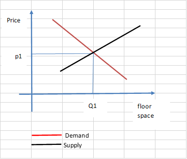
The red demand line intersects with the black supply line. Q1 quantity of floorspace is provided at P1 prices. All good.

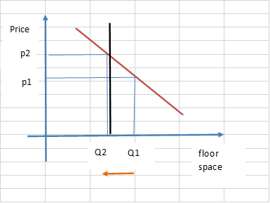
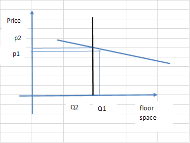
Now we introduce a (valid, well justified) constraint on supply. The black supply line is vertical (fixed) rather than sloping.

The price of the floorspace increases from p1 to p2, while the quantity supplied reduces from Q1 to Q2.

But this might be called a closed or static city model. Supply is fixed, there are no compensating actions; development cannot shift location within the city due to the constraint, for example.

What happens when we have a more dynamic city where things can shift and adjust?

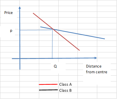
We need to start with two different types of floorspace: Class A central city and Class B fringe office space, for example.

Then we assume the following two demand ‘curves’. They have  different slopes. Class A office space is more willing to pay higher prices to be closer to the centre, so the demand curve is steeper than the Class B demand line. Where the two demand lines cross over is the edge of the CBD.

What happens if the supply of Class B floorspace is constrained? First we have to assume what the non constrained supply curves for Class B space may look like. In the following graph I have ‘grayed out’ the Class A office space demand and supply curves, and left in the (assumed) Class B office space demand and supply curve.

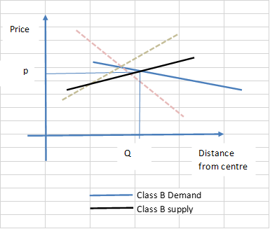
So quantity Q of Class B space at price p.

Then we add in the vertical constraint. The quantity of Class B space goes down from Q1 to Q2 (as a movement to the left means less space), and price of Class B space increases from p1 to p2.

What happens to the unmet Class B office space demand? There is demand for Q1, but supply is limited to Q2. What happens if that supply gets transferred to the central area, to the Class A floorspace area? The Class A area has only one constraint on the supply of office space. No height limits apply, so the Class A area can go higher. However the Class A area cannot expand out any further.  

We also need to assume that the unmet Class B space demand cannot go the ‘other way’; that is, shift to being further away from the centre, into the next ring out. For example, let’s assume that the next ring out is residential zoning. It may also be possible that the unmet Class B demand shifts to a different city altogether (like Hamilton).

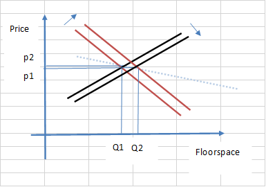
The following graph shows the shift in demand for Class A space (the two red lines) in response to some displaced demand from Class B office space area.

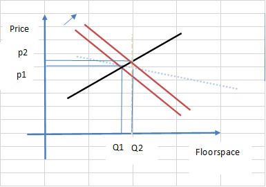
In this case the demand for Class A space shifts outwards, so the quantity supplied increases from Q1 to Q2, but price goes up from p1 to p2.

But if the Class A space supply can increase (more height for example), then the supply curve may shift, and prices might not change that much. In this case the supply line shifts to the right a bit. Prices may go up a bit, depending upon the slope, but maybe not as much if the supply curve stays static.

So overall, the constraint has three effects:

1. The supply of Class B space is less than what is demanded and a bit more expensive for all those offices space consumers in the Class B space area;
2. Class A space expands to accommodate the office space that can’t get into the Class B area. This extra demand may increase prices, less so if supply can also expand easily;
3. The displaced Class B space consumers who occupy Class A space end up paying more for their office space than might otherwise have been the case, or perhaps the Class B office space users need to consume less Class A office space than they might otherwise do, to keep their costs down.   

Now time to turn to my imaginary city and its land values and building heights.

In my imaginary city, presumably there are some land value changes as a result of the suppression of demand in the second ring out, but also changes from some of its relocation to the central ring.

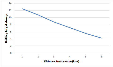
If we start with the land values for the first two rings of my made up city, then we get the following graph. The graph has time periods on the horizontal axis. As time goes by and the city grows, then land values steadily rise.

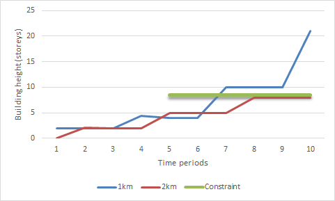
I then turned those land values into building heights (using a basic assumption of $100 of land value units supports 1 storey of floorspace). Taking into account that buildings last for 3 time periods before they can redeveloped, then I get the following building height profile.

Now the question is what may happen should the 2km ring of development be constrained in some way.

The following diagram has a building height constraint of 8 storeys applied to the 2km ring; a constraint that has effect at time period 8. Rather than be 11 storeys in the unconstrained model, in this case buildings are 3 storeys less in height.

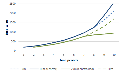
The next graph returns to land values. It suggests a ‘flattening’ out of the 2km land value curve, in response to the 8 storey constraint. Perhaps land values continue to rise, but to a lesser extent than the unconstrained model.

Over time, there is quite a wedge between what the 2km curve might have looked like without the constraint (the dashed 2km line) and the constrained line.

Now let’s assume that most of the 2km floorspace demand is displaced to the 1km floorspace area. The value of land goes up as demand increases.

This is not a one-for-one shift, as land values in the 1km ring are higher than the 2km ring (in my case about 20% more). So demand for 3 storeys in the 2km ring might translate into demand for 2.5 storeys in the 1km ring, if the amount that tenants pay in rent stays the same. 

Land values in the 1km ring increase as supply of floorspace responds to demand rises. Overtime the wedge gets bigger. 

Back to the opening diagram, part of the difference in land values between the inside and outside of the constraint could therefore be from displaced demand.  Not all of the difference is a cost from suppressed supply. The reduced land value from the constraint is probably not off-set by an equal amount from increase in land values on the other side of the constraint, but there is likely to be a bit of a shift. 

So with the constraint in place and some transfer of floorspace demand, we can make the following comments:

Area (ring)	Amount of floorspace	Land values	Floorspace rents
1km - unconstrained (Class A area)	More	Higher	Higher, depending upon supply
2km - constrained (Class B area)	Less	Lower	Higher

Landowners in the unconstrained area are likely to see a benefit, but landowners in the constrained area will see lower values than might otherwise be the case.

Building occupiers are likely to see increases in prices/rents in both areas, and as mentioned, Class B office space occupiers are likely to have to accept higher prices or smaller premises if they have to shift to Class A office space areas.

The above are the 'costs', not the 'benefits'. Working out the benefits of the constraint is beyond me. There is the direct benefit, but there may be other, off-setting benefits from more floorspace in the Class A area:

• Public transport services may be better. Big investments like the Central Rail Link in Auckland may be made sooner if there is more floorspace . This investment in transport accessibility benefits all landowners and tenants. 
• Some redevelopment of sites may be brought forward if there is more demand
• The Class B occupiers may fill up ‘hard to rent’ areas in the central area. 
• The unconstrained area may be a busier and more lively place with more cafes and lunch bars, helping to generate more vitality. 

On the other side of the coin, less floorspace in the constrained area may reduce the vitality of that area.

Perhaps the short answer to the initial question of what are the implications of a constraint is that it is hard to unravel all of the changes that go on. The other point is that for every constraint imposed, does there need to be some sort of alternative location provided? That alternative may not be perfect, but at least there is some form of 'compensating' action. 

However, overtime, as the wedge between what might otherwise happen and what does happen in the constrained area gets bigger, it may be harder to put in place these compensating actions. 

More on on-site car parking and decision making

A couple of blogs back I started to look at the question of how to assess the effects (consequences) of an on-site parking shortfall for a housing development in a Special Character Area in the inner suburbs of Auckland. I want to do this to better understand decision making, rather than look at the details of the specific case.

I started with the proposition that I would try to understand the nature of the effects and the state of the environment impacted by those effects. Next step would then be to consider the significance or consequences of the effect by looking at the relevant planning documents.
The case study involves a 19 dwelling development with 9 on-site car parks, a short fall of 10, based on the  Auckland Unitary Plan requirement of 1 on-site space per dwelling.

First, I tried to gauge car ownership based on 2013 stats data on the number of cars per dwelling, taking into account bedroom numbers and locality.  I also tried to guess the 'state' of the on-street parking resource in the area.

I came up with the following 'effects' of the proposed development:

1. Number of extra cars in the neighbourhood = 22
2. Number of extra cars looking for kerb side parking = 13
3. Reduction in cars in the region due to inner city location compared to if dwellings were located on the edge of the region = 4
4. Higher rates of public transport use (around a 15 percentage point increase) and lower vehicle kilometres travelled (perhaps 20% less) compared to if dwellings were located elsewhere
5. Increased pressure on existing residents in the area to find street parking spaces and hence more pressure to accommodate cars on site, possibly affecting special character values of the environment. 
6. There may be increased demand for car sharing type services, if parking gets harder to find and so people decide to get by with fewer cars. 

Something I missed was the amount of developable space 'freed up' by not having so much on-site space taken up by car parking. Each car parking space occupies about 25 to 30 square metres of land area by the time you take into account manoeuvring area. 19 units are proposed requiring 19 car parks. 9 on-site car parks are to be provided, meaning that space for 10 cars would need to be found. 10 car parks might occupy up to 250 to 300 square metres of space. This is probably equal to at least 2 small dwellings or 1 larger dwelling So a further consequence of having less on-site car parking is having two more dwellings to add to regional housing supply.

The effects are a mix of transport, amenity, and urban form and function effects. They span local and regional scales. The effects are not just about local on-street parking demand and supply. This is pretty typical of RMA and urban planning matters - things are connected.

They are not effects that are in addition to, or more than what might otherwise be expected. They are the 'full' effects, as best as can be estimated. However I did speculate what might be a realistic alternative proposition to give some context to the effects.

The state of the receiving environment is harder to gauge. I estimated that street parking was in high demand, and that over time street parking is coming under pressure through gradual infill and redevelopment, although car ownership rates are dropping. There is also demand from visitors to nearby commercial areas and commuters. I also speculated that the surrounding urban environment was sensitive to pressure to incorporate more on-site car parking on sites, with older villas and bungalows present.

The  consideration of effects has lead to a couple of preliminary thoughts about decision making, and before looking the AUP it is worth exploring these a bit more.

To begin with, the AUP has set in place one decision making 'trigger'. Put another way, there  would be no need to consider all these effects and their connections if either of two conditions existed:

• Firstly, if the development provided the required number of on-site car parks, then all of the other related effects of transport, urban form and amenity fall away from consideration, even if the development adds to street parking demands or fewer houses are built; or
• Secondly, if there was plenty of on-street parking available, then the pressure created by the development for more use of street parking doesn't matter, and again there is no need to consider the other related effects and their consequences.

Decision making triggers are supposed to  be set so that when some condition is exceeded, then investigation and action is needed. Whether the plan has the right trigger is not clear to me. Decision making trigger points should be based on the boundary between a stable (or desirable) and an unstable (or undesirable) environmental state. For example, would a better trigger point be that when street parking reaches 70% saturation, then developments that do not provide on-site parking need to be looked at in more detail? But then that is not easy to measure.

Where there are multiple objectives involved (urban form, transport, amenity) and there is some competition between the objectives, then does the decision making trigger point need to involve some built in (or apriori) trading off between the variables?  Has this been done?

Furthermore, if the decision making conditions are triggered, then there is a presumption that the pressure exerted on street parking from less on-site parking needs to be 'managed' in some way to maintain the stability and integrity of the system or environment. This is a big assumption. In one conception, street parking is a public resource, and like all public resources, it is a resource that can be easily over used to the detriment of all. Is there a value-based judgement to be made that street parking should be 'allocated' fairly?

Another  viewpoint may be that overuse can see flow on or spill over effects to amenity and the quality of the built environment in the area. But equally there are a bunch of benefits to the regional housing market and the regional transport system from allowing more housing in inner city areas where street parking resources are under pressure. 

Final question: do you always need an alternative scenario to help set the effects in context? Decision making theory talks about the importance of the 'counter factual' - for example the environment without the development in place. Something will happen on the site in question, but what might happen? It is important to describe the counter factual accurately and to use it consistently, as the positive and negative effects of the development should be placed in context against the counter factual. Identifying the future without the project is often not straightforward, in particular where the environment is likely to evolve overtime. Does the plan enable a good estimate to be made of the future without the project?  The plan may set a clear 'permitted baseline' which can be taken into account, but what if that baseline is not clear, or is so limited in extent it doesn't provide a realistic 'counter factual'?

Is it time to allow for more building height on the edges of the CBD?

Is it time to allow for more building height on the edges of the CBD, outside the motorway ring? Is somewhere like Newton, with the new CRL link in place,  ripe for going up in a major way (setting aside volcanic viewshaft issues) ?

Generally we see the city as having the tallest buildings in the middle, with building height dropping off towards the edges. This pattern reflects land values, with the highest values being in the middle of the city. But the age of existing building stock means that re-development is often patchy and concentrated in some areas, but not others, creating a jagged rather than smooth city skyline.  The durability of capital means that the newest, tallest buildings may not always be in the area of highest land value.

The following is a thought experiment after reading Bruecknar’s book: Lectures in Urban Economics. In his book Brueckner has a chapter on the durability of capital and its implications for patterns of redevelopment.

If we start by assuming  that buildings have a useful life of 75 years, then the height of the building will reflect the land values at the start of the building's life (ie 75 years ago), not what land values might suggest after 50 or 60 years of existence. When the building ends its useful life, and it is time to pull it down and rebuild, land values will have changed (assuming a growing city). The new building will likely be quite a bit taller than what previously stood on the site.

Lets further assume we have a city that starts from scratch. In the first 25 years of its life it expands to fill a 1 km radius. The average age of buildings in 12.5 years. The 1 km radius is not a set number, it is just a convenient figure. It could just as well be 1 mile or 1 city block.

The below table has the first growth period.

Table 1; the first 25 years

	Years 0-25
Distance 1 km
	12.5 average age of buildings

The city continues to grow over the next 25 years. The city expands out another 1 km. The buildings in the central km get older, their average age is now 37.5 years, while the buildings in the next ring out are on average 12.5 years. 

Table 2: The next 25 years

	Years
Distance	0-25	25-50
1 km	12.5	37.5
2 km		12.5

This pattern repeats itself over the next 25 years. A further 1km is added to the city's  radius. The buildings in the central 1km are now 62.5 years old, and getting towards the end of their useful life. 

Table 3: Up to 75 years

	Years
Distance	0-25	25-50	50-75
1 km	12.5	37.5	62.5
2 km		12.5	37.5
3 km			12.5

What happens in the next 25 year period? 

The city expands outward more, but the first 1 km is redeveloped. The average building age exceeds the 75 year life span. Here the average age of the building drops back down to 12.5. 

Table 4: 0-100 years 

	Years
Distance	0-25	25-50	50-75	75-100
1 km	12.5	37.5	62.5	12.5
2 km		12.5	37.5	62.5
3 km			12.5	37.5

If we repeat this pattern some more, then by 5th, 25 year period, the buildings in the second ring out (2 kms) are redeveloped. 

Table 5: Redevelopment 

	Years
Distance	0-25	25-50	50-75	75-100	100-125	125-150	150-175	175-200
1	12.5	37.5	62.5	12.5	37.5	62.5	12.5	37.5
2		12.5	37.5	62.5	12.5	37.5	62.5	12.5
3			12.5	37.5	62.5	12.5	37.5	62.5
4				12.5	37.5	62.5	12.5	37.5
5					12.5	37.5	62.5	12.5
6						12.5	37.5	62.5

By the 7th period, the buildings in the first 1 km are ready for their second round of redevelopment. There is a successive wave of redevelopment, with the highlighted cells in the above table being the periods of redevelopment. 

Of course development and redevelopment is never this tidy a process, but it is the concept that counts at this stage. 

If  we then assume a land value increase in each 25 year period as the city grows, then we begin to see how building height may not have a smooth profile from the centre to the edge. 

The table below lists land values - these are made up values and are not realistic figures. They assume a constant rise in values. The highest values are always in the middle of the imaginary city - in the first 1 km.  

Table 6: Made up land values ($ per sqm)

	Years
distance	0-25	25-50	50-75	75-100	100-125	125-150	150-175	175-200
1	$200	$260	$340	$440	$570	$740	$960	$1250
2		$220	$290	$380	$490	$640	$830	$1080
3			$237	$310	$400	$520	$680	$880
4				$248	$320	$420	$550	$720
5					$255	$330	$430	$560
6						$257	$330	$430

If it is then assumed, for the sake of simplicity, that each $100 of land value equals 1 floor on a building, then you might assume that by to 8th period, with the city getting about 200 years old, then the city's height  profile might look like this: 

Figure 1: Building height based on land value profile

I know this is not a very realistic profile, as usually there is a steep drop off of land values (and hence building height) close to the centre, then a more gentle decline thereafter. However, again it is more the concept which is important. 

If we take into account age of buildings and likelihood of redevelopment then we are more likely to get a pattern like this for the 8th time period.

Figure 2: Building height based on land value and age

This is because building height is determined by the land values at the start of the building’s life, and depending upon the sequence of growth, ageing then redevelopment; the highest land values may not be in the area with building stock ready to be redeveloped. 

The above graph is based on the following figures, which are of the assumed number of storeys. Average building height is constant for three, 25 year periods reflecting the assumed life of a building being 75 years,  with that height based on the made up land values in Table 6 in the first 25 year period.

Table 7: Assumed height of buildings

	years
distance	0-25	25-50	50-75	75-100	100-125	125-150	150-175	175-200
3	2	2	2	4	4	4	10	10
6		2	2	2	5	5	5	11
9			2	2	2	5	5	5
12				2	2	2	6	6
15					3	3	3	5
18						3	3	3

So, is it possible, given the timing of redevelopment pressures, that the building stock on the edge of the CBD is more likely to redevelop than the stock within the CBD?

Certainly if we look at the Auckland CBD, after a period during which a lot of building development occurred down along the waterfront area, there are signs of building activity occurring in the mid CBD area, with some very tall towers now proposed close to the mid town Aotea area.

Actual land values drop off quickly between  the waterfront area of the CBD and the Newton area and so it is unlikely that Newton will see taller buildings than downtown. Having said that, CRL is likely to see some dispersal of office based activities to edge of CBD areas as the upgraded rail system modifies accessibility profiles.  Time to re look at building heights in places with high land values and older building stock?

Perhaps the more interesting question is the extent to which the above patterns of age of buildings and land values may influence patterns of redevelopment in residential areas. Capital (houses) can be very durable if there are strong emotional values attached to houses, for example, while often redevelopment is slowed not by the age of buildings, but by the fragmentation of land.